Make a graph of data
This tutorial will take you through the steps of creating your first graph in Grafana, with data stored in InfluxDB.
It assumes that you have data already written in the database, as described in Store data in database.
We will go through the steps:
- Setup a datasource
- Create a new graph
Everything will be done in Grafana, which (if you have the playground running on your computer) should be accessible at http://192.168.99.100:3000.
Open a browser and go to the adress above to get started!
This should take you to a login screen, the default login is:
User: admin
Password: admin
Now we are ready to get started!
Setup a datasource
First we must define where Grafana will get the data.
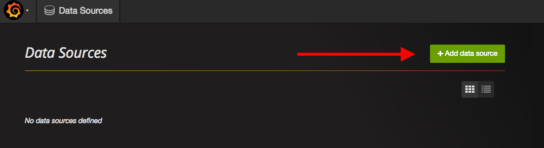
Press the menu in the upper left corner (under the Grafana logo), and then Data Sources.

And then we are going to add a new data source.
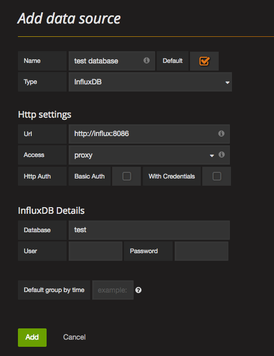
The settings that we care about right now are.
- Name is just something to call the datasource.
- url is the ip-adress/hostname where grafana can find influxDB. In the playground, we use docker container linking, so influx will be available at the Url
http://influx:8086 - Database is which database that we want to get the data from. In the Store Data tutorial, we used a database called test, so we are going to use the same one here.
When your settings looks like below, hit Add!
If you get a message saying

You are good to go!
Create a new graph
First we need to create a dashboard where our graph will be.
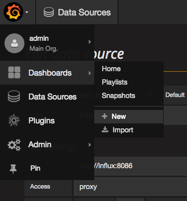
Under the Grafana menu again, press Dashboards -> New
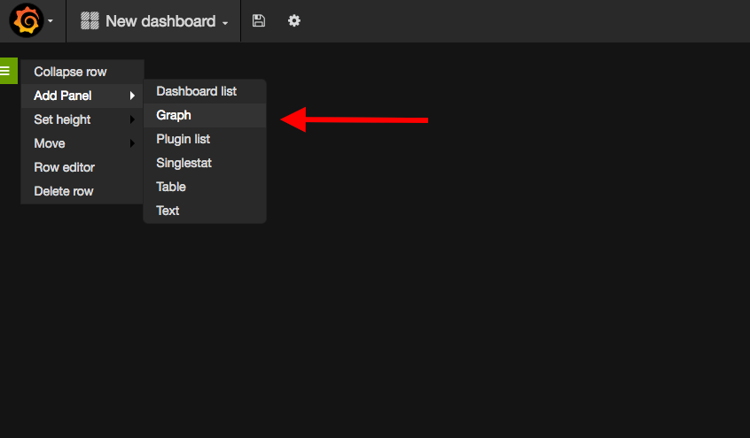
Then comes probably the most confusing part of all our tutorials. Hover the tiiiiiny green sliver way over to the left to expand the menu of the first row of our dashboard (which is empty though, so you can't really see that it is a row).
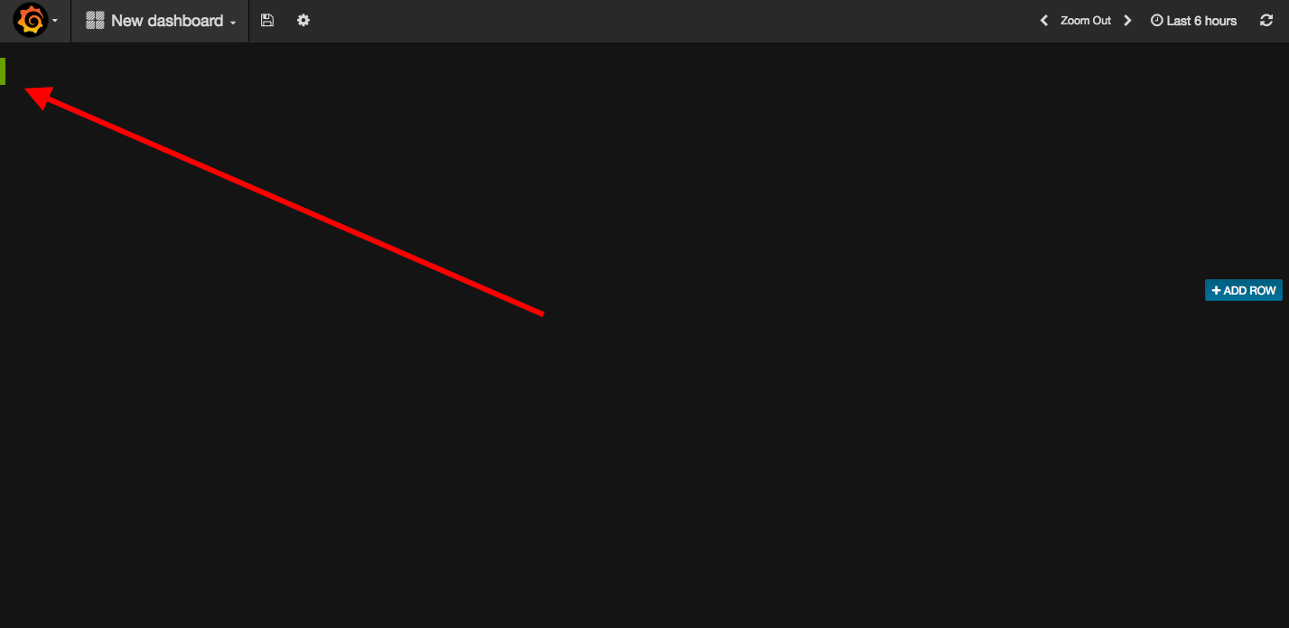
Select Add Panel -> Graph
If not already selected, set the panel data source to the datasource we just created.
Then press the long row with the query to expand the details.
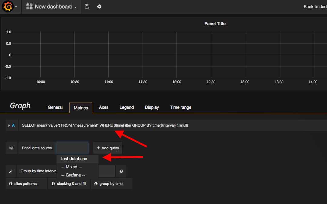
Here we can set how Grafana will get the data from influx, and how to display it.
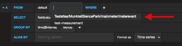
Press select measurement and choose the measurement where you have the data points, in our case Testsites/MunktellSiencePark/mainmeter/meterevent.
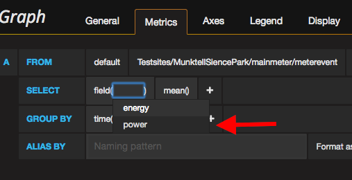
Next, press the field(value) on the row below, and we can see what fields that are available in this measurement. power will give the most interesting graph, so we select that one!
And that should be it! We should now see a graph of the data in the panel, that looks something like this:
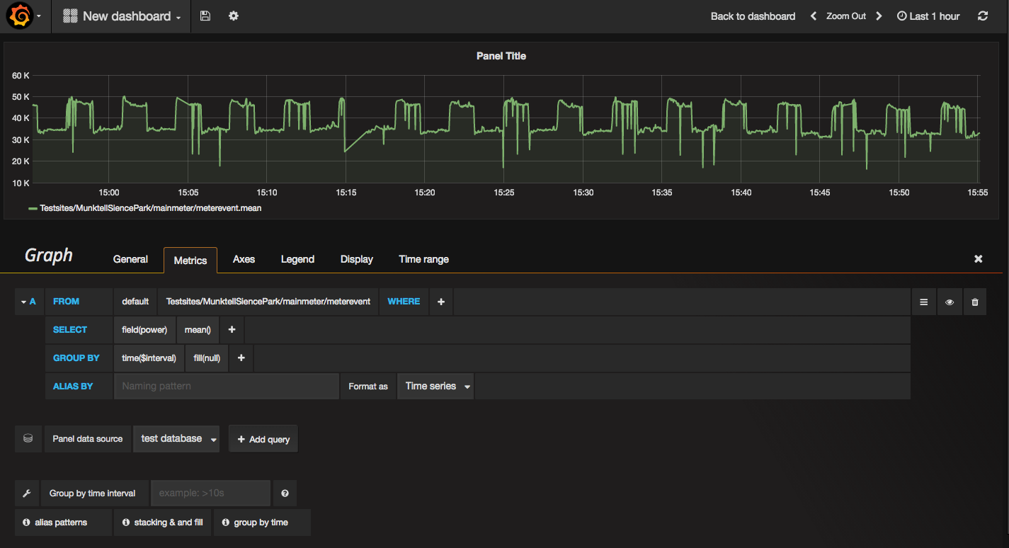
Yours might look a bit different depending on how much data you have, what sort of data it is etc.
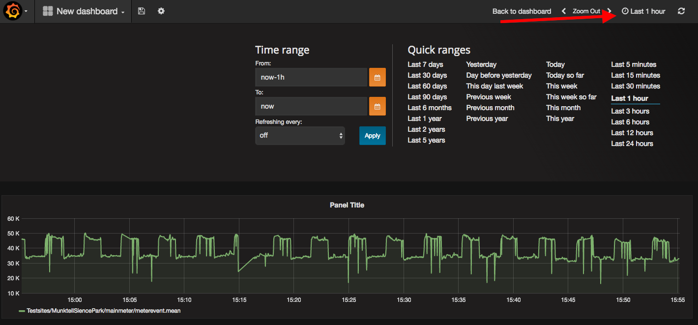
The scaling also matters! To change the scaling of the dashboard, use the settings in the upper right corner.
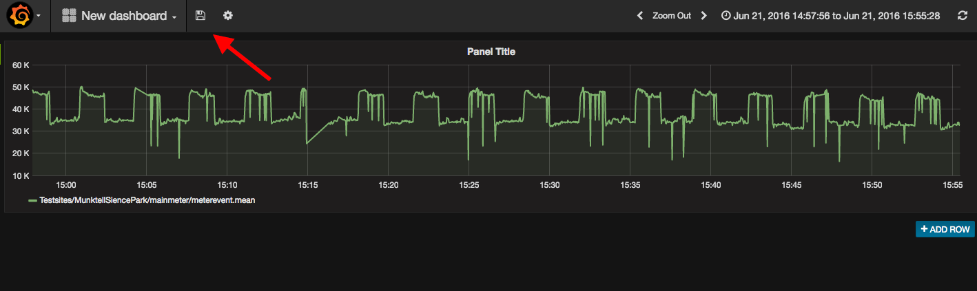
The last step is to save the dashboard! Press the little floppy icon in the menu bar.
There are lots of other settings you can change to customize the graphs. Play around in Grafana to see what you can do!
If you want to view an example of how Grafana could be used, there is an official instance of it running at https://op-en.se/graphs.
Next
TODO.
What should be next?